Sorting Algorithms and Optimizations

Hello netizens of GitHub and beyond, I am Dang, and this is my blog about how a simple argument between me and my friends turned into my course project. So, me and my friend Mahesh were arguing about who’s laptop is better. A little bit of context here: we both were taking Computer systems Architecture class and we were both hardcore FIFA fans. While discussing about the system requirements to run the game, we got into an argument of whose gaming rig could better run the game at higher resolution and fps.

I had an i5-7300HQ designated as Kaby Lake architecture on my rig whereas my friend Mahesh had an i7-8705G with Radeon RX Vega M GL which is supposed be some new integrated CPU-GPU on the same chip architecture also called Kaby Lake-G . Being stubborn as I always am, I thought my i5 could outperform his i7. By now another friend of mine, Anantvir, joined our discussion and his rig was a i7-8750H, a designated Coffee Lake chip architecture.

We three decided to do a project for our Computer Architecture class by comparing laptop architectures by running different algorithms at different optimizations to see how each of our architectures would perform. The reason we decided to test our machines using sorting algorithms is their key role in many real-life applications. Almost any multi-tiered application uses search and sort algorithms in some form or another. Another reason was that we could truly test the processing time of our computers without any communication or network overheads distorting our results. (Also, it was the easiest way to find out the capabilities of each processor.)

As we were setting about to get started on our project, we began learning how optimizing code differently can lead to different results on different architectures. We started out by writing our code for the different sorting algorithms on C/C++ as our initial goal was to run these sorts using the GNU Compiler Collection (GCC) or G++ and its array of different compiler optimizations. There are 8 different valid -O options one can give to GCC, though there are some that mean the same thing: • -O (Same as -O1) • -O0 (do no optimization, the default if no optimization level is specified) • -O1 (optimize minimally) • -O2 (optimize more) • -O3 (optimize even more) • -Ofast (optimize very aggressively to the point of breaking standard compliance, messes up floating point calculations) • -Og (Optimize debugging experience. -Og enables optimizations that do not interfere with debugging. It should be the optimization level of choice for the standard edit-compile-debug cycle, offering a reasonable level of optimization while maintaining fast compilation and a good debugging experience.) • -Os (Optimize for size. -Os enables all -O2 optimizations that do not typically increase code size. It also performs further optimizations designed to reduce code size. -Os disables the following optimization flags: -falign-functions -falign-jumps -falign-loops -falign-labels -freorder-blocks -freorder-blocks-and-partition -fprefetch-loop-arrays -ftree-vect-loop-version)

Of these 8, we chose to use O0,O1,O2,O3,Os and Ofast. Later, we would go on to add -fopenmp to this list of compiler optimizations. The following table explains, in a crude way how these optimizations affect the code, execution and compile times (https://www.rapidtables.com/code/linux/gcc/gcc-o.html).

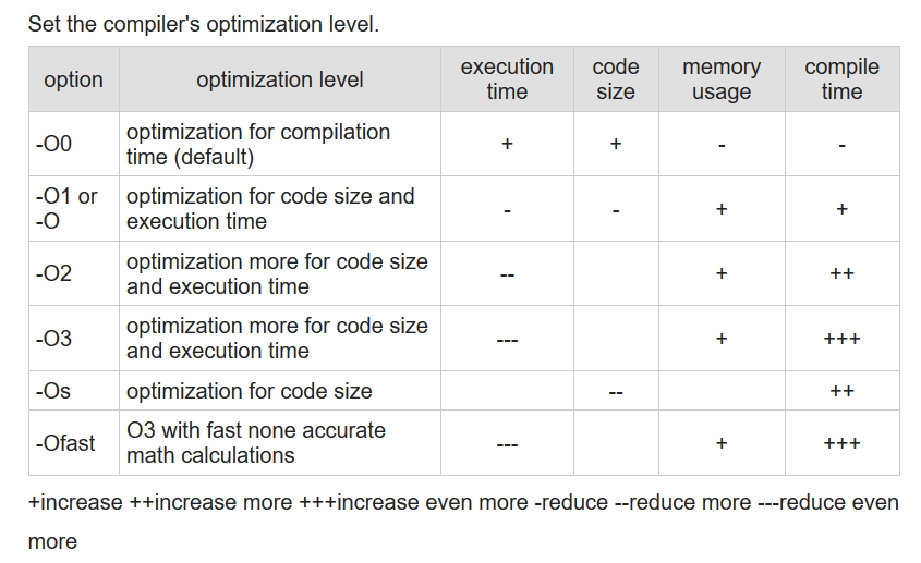
We also found this table to be very helpul while understanding the flags associated with optimizations.

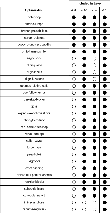(https://www.linuxjournal.com/article/7269).

A code can be optimized in two ways: Write a code which is pre-optimized or let the compiler do it for you. Humans aren’t very good at solving/computing complex and sequential data. There a million ways to write a piece of code, and as you go into low level languages, the more sequential it becomes and the harder and longer the code becomes. In this day and age of such huge codebases and Big Data applications, with an exabyte of data being produced every day around the world, we need to focus on making applications which can focus on cleaning and processing these huge dumps of data. Leave the optimizing to the compilers. A compiler when given a code and a directive on how to optimize the code, uses several different techniques to achieve this. For example, in the GCC, O1 applies 30 optimizations to the given code. This makes the work of the programmer much easier and the code much efficient. So, with our compiler, optimizations and code ready, we were ready to begin! We started out with a 5k int type data set, but the clock() function in time.h library couldn’t even measure the time it took to execute the sort. So, we steadily increased our data by 10k each iteration. After crossing 50k we began seeing time being registered the clock() function. So, we tested 50k,100k,200k and 500k datasets for good measure. What we observed was that the increase in execute time as we increased the datasets was almost linear, so we decided on plotting the 100k dataset as it showed us the most difference in different optimizations and on different machines. Similarly, we ran the code on the same datasets but used float type datasets.

Then we scaled the project to a total of 6 algorithms. The results can be seen below:

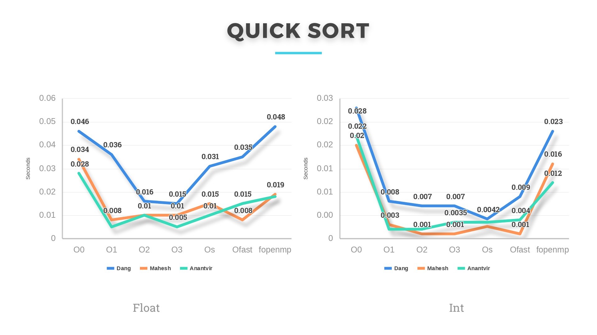
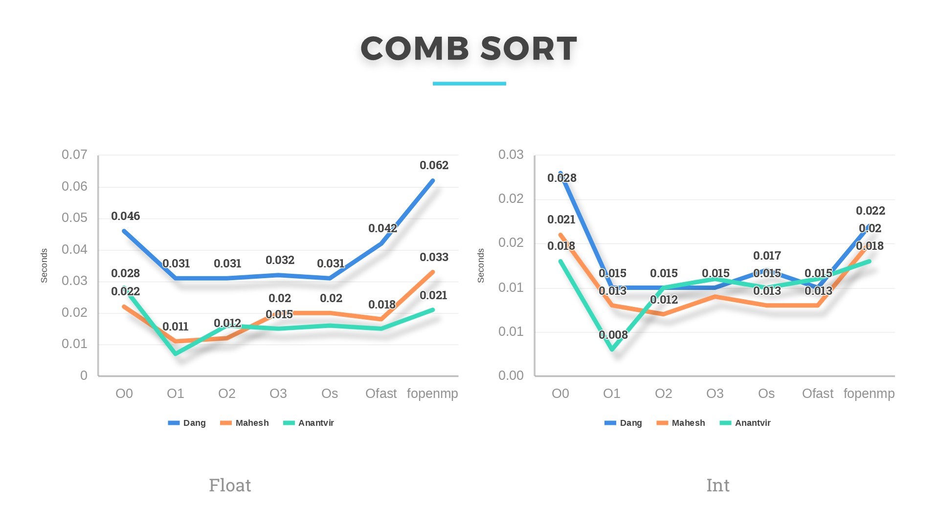
Combsort and Quicksort have worst case complexity of O(n^2) and average case complexity of O(nlogn). They performed in accordance with their complexity. If we randomize quicksort algorithm, then the pivot will be chosen randomly from the given distribution and the expected running time will be linear E[T(n)]=O(nlogn). Its is then possible that quicksort will perform comparable to Heapsort and Combsort.

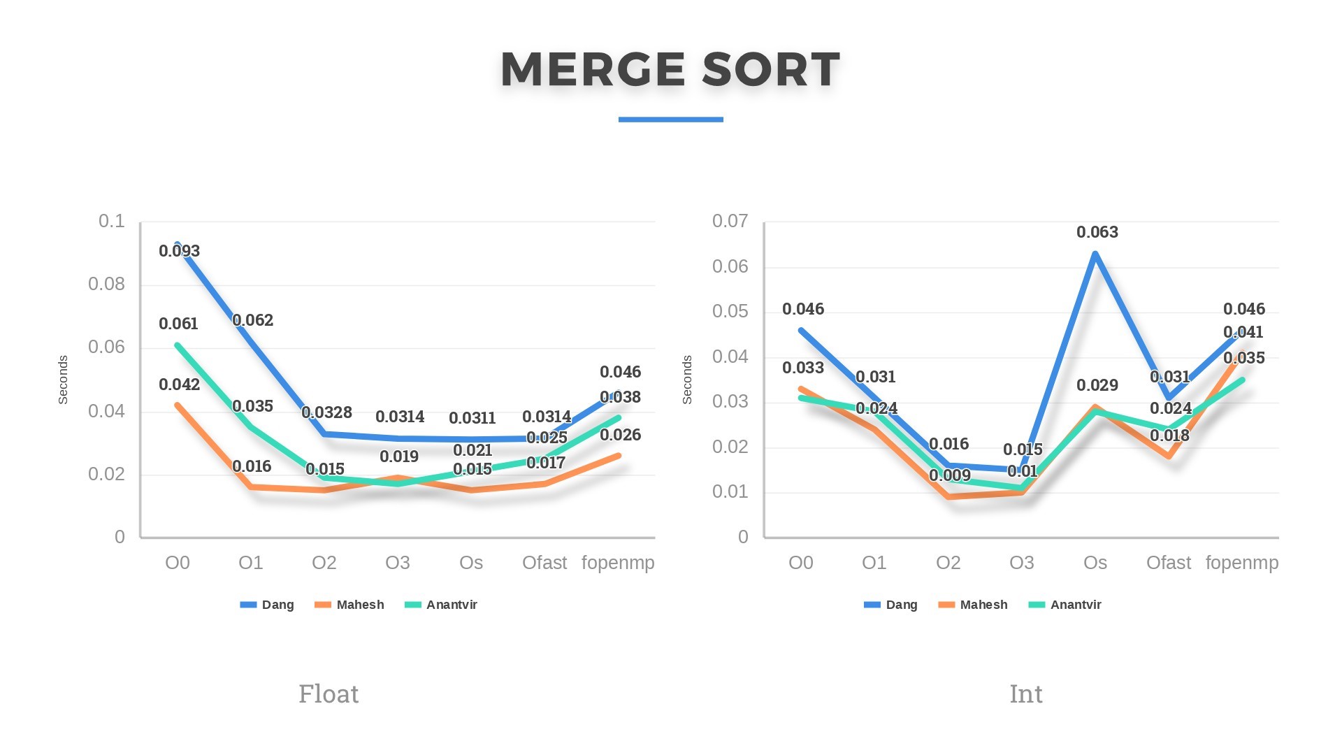
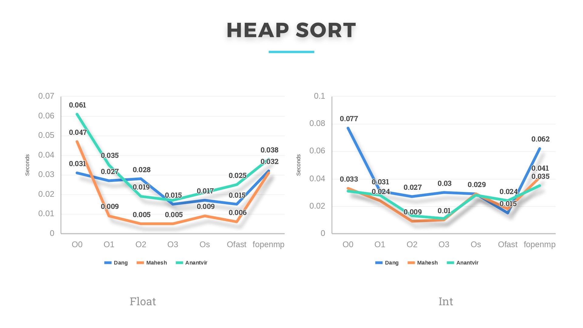
Heapsort and Mergesort, both have an average and worst case complexity of O(nlogn). Both these algorithms perform the best of all 6 algorithms in our analysis. For datasets >10000 integers and floats, Heapsort performed a little better. Also, there is a difference in running time of these algorithms every time we ran them on the same machine. This might be due to other applications running in the background occupying cache and utilizing more of CPU.

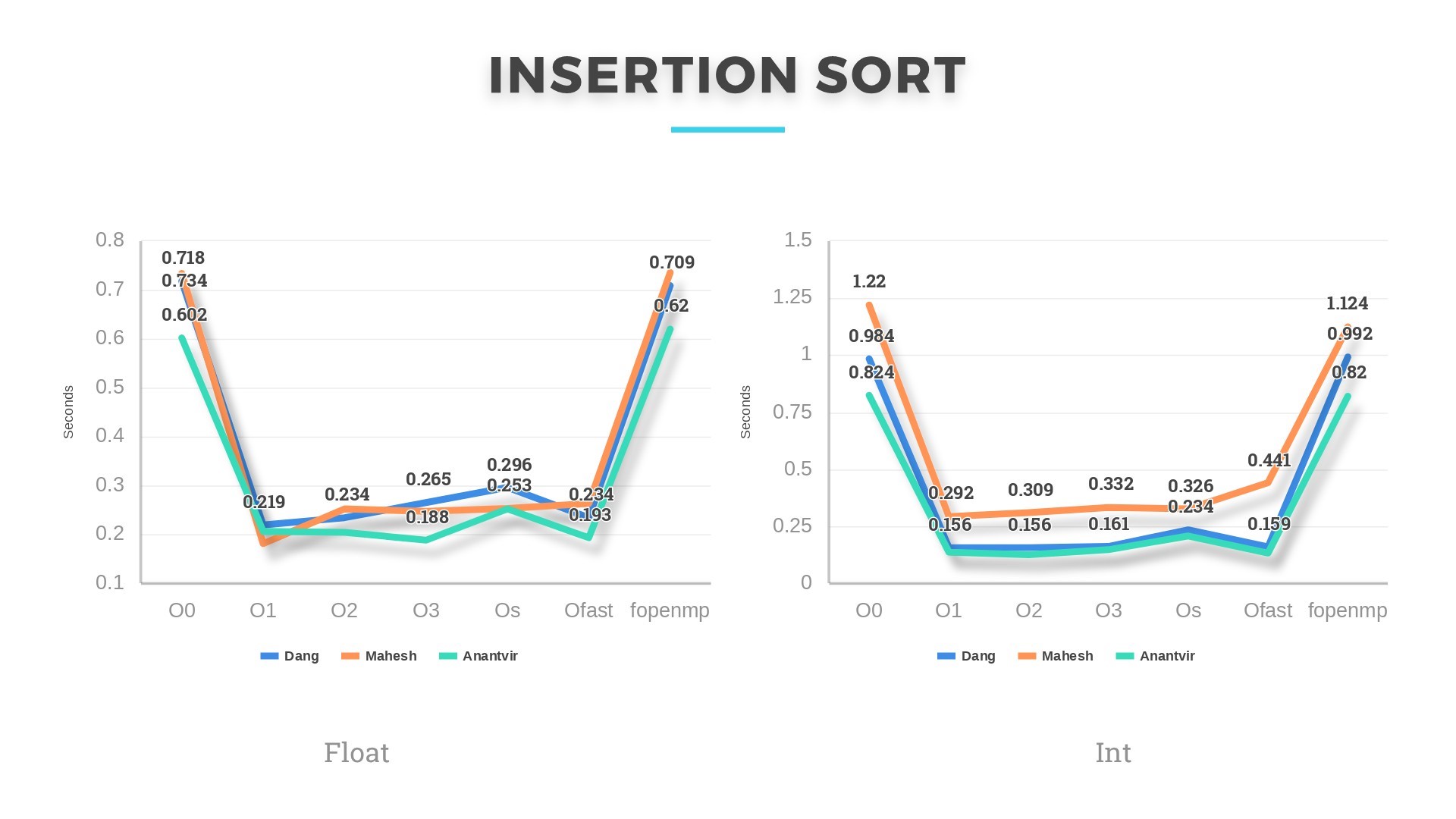
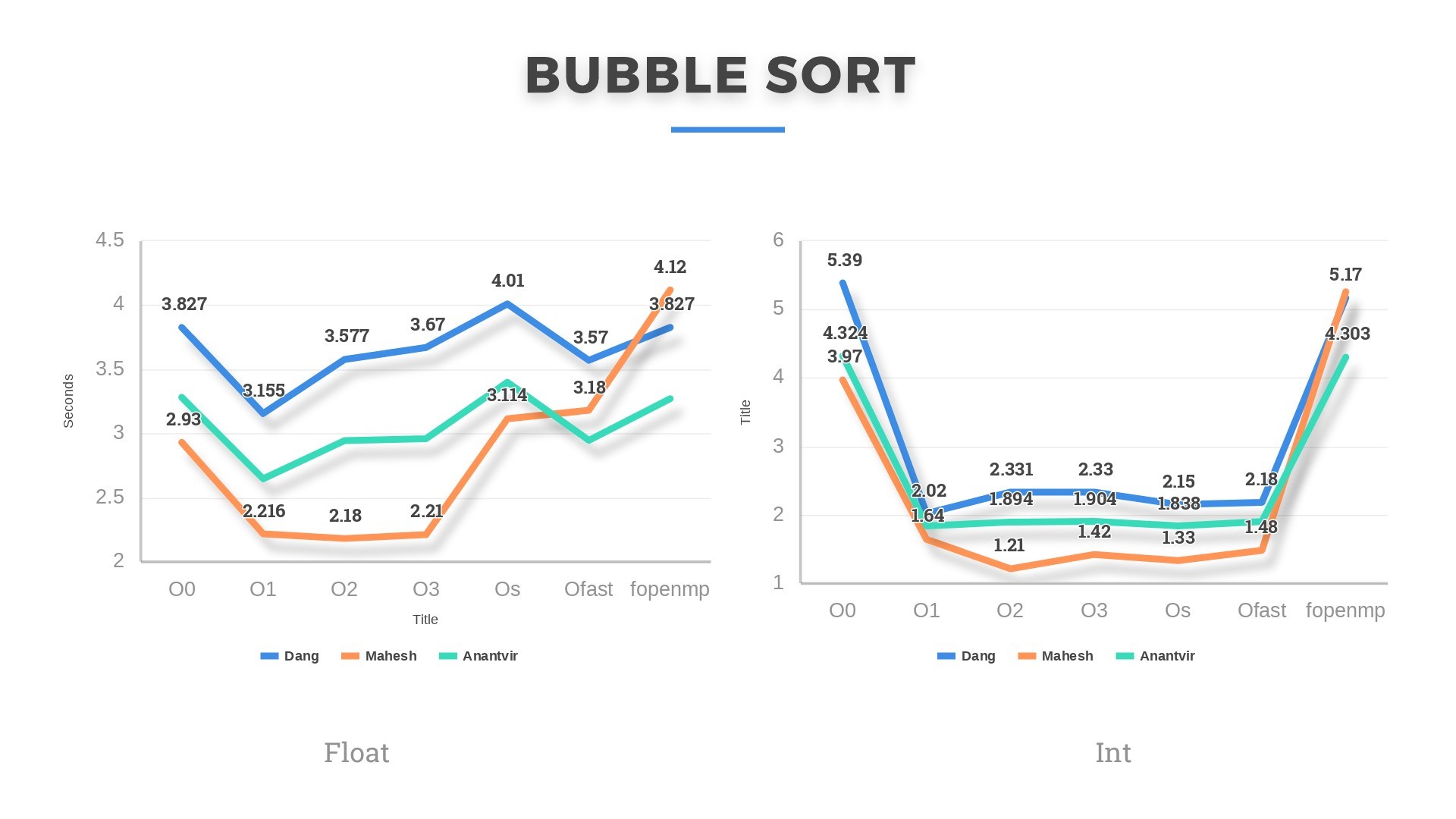
Bubblesort and Insertionsort, having the highest average and worst-case complexity of O(n^2) were the slowest of all. In some cases, Bubblesort even ran for 13-14seconds on 50k floats. This shows that comparison-based sorts are never a good choice if input size is large enough. Although slow, but these algorithms gave the most speedup under optimizations. In some cases, the running time even reduced by 60 %. Performance Outcome: We learned that my machine performed slowest of all except in the case when Insertion sort is run on Integer dataset. Mahesh’s machine, having the highest base clock frequency of 3.1GHz was the fastest of all except in Insertion sort (both float and integer) and Combsort (float only). He was bragging about this and then we were decided to parallelize the algorithms. Mahesh was quite confident this time as well that his laptop will be the best among the three.

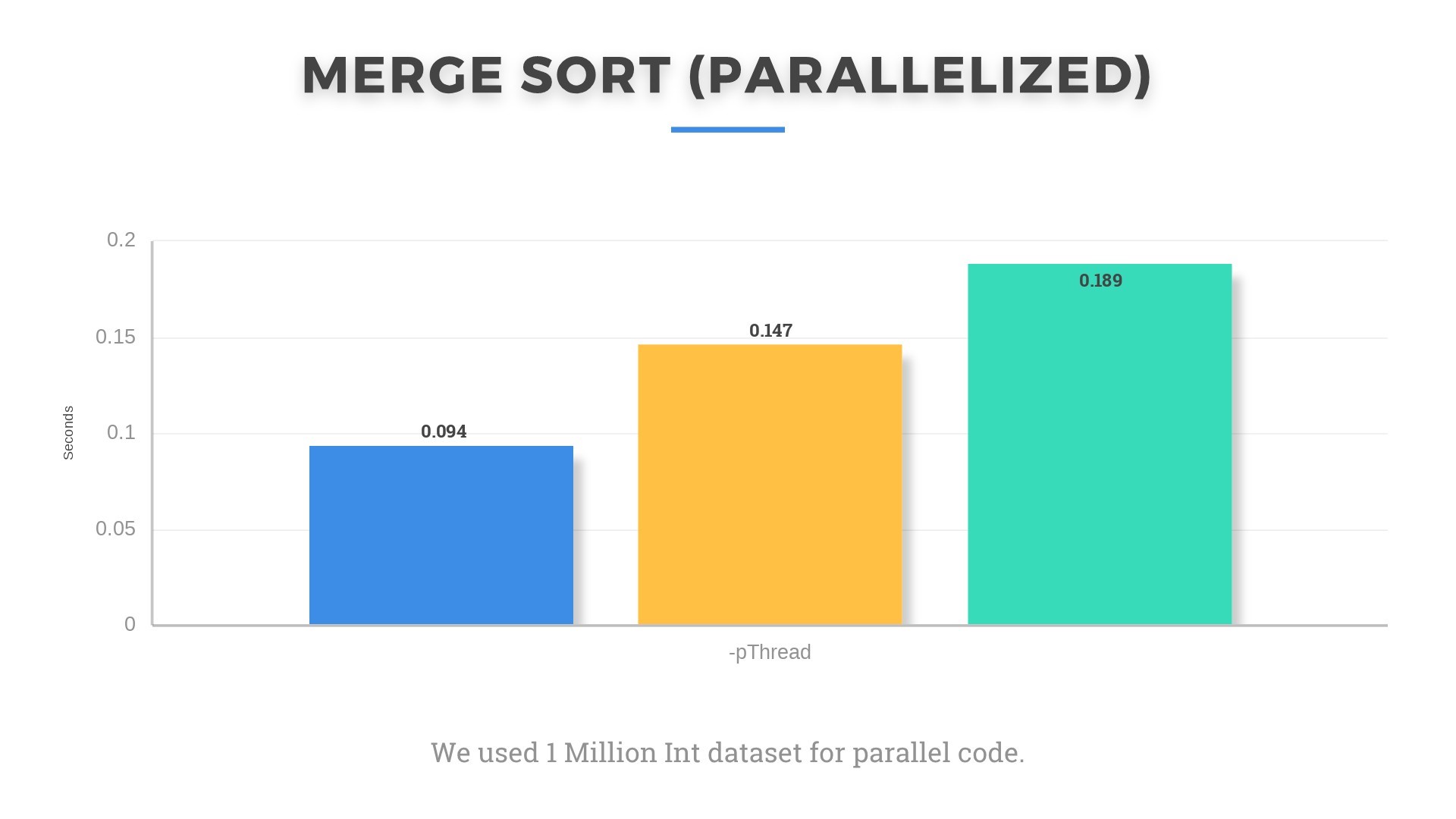
Surprisingly, my laptop gave better results when we parallelized the Mergesort code and ran it on input of 1 million integers. Although I believe that running it only on 4 threads gave me the edge as his could also run on 8 threads, but he didn’t know how to do that(OWNED.). Anantvir’s machine also underperformed on the parallelized algorithm. We were not able to figure out the reason for this oscillation of performance. We think it might be due to different background processes and threads running in OS at the time. The clock frequency also keeps changing randomly as can be seen from Task Manager in Windows 10 according to the CPU and memory utilization. Even under small loads such as multiple tabs open in Google Chrome, base frequency increases to 3.9 GHz and reduces to 1.5-1.8 GHz when browser is closed. Such small things make significant impact on running times. Even being plugged in changes things as turbo boost was set to active only when plugged in. Weird things are happening under the hood. Takeaways: 1) Working of all sorting algorithms. This is the first time we actually implemented the algorithms. 2) Real world applications of sorting. It doesn’t just sort numbers. They are widely used in day to day tasks like Microsoft Excel, Database sorting, programming language libraries sorting. They have wide use in Computer Vision where objects are sorted by their distances to improve rendering performance.
3) Working of compiler optimizations. We did not even know until we started the project that code can be optimized by such optimizations. In addition to Loop blocking, Loop interchange and other optimizations studied in the course, we were able to understand the working of many new optimizations, how they run under the hood to exploit spatial and temporal locality. 4) Knowledge about actual speedup obtained by these optimizations, on what algorithms, what data size, percentage increase in performance etc. This might help us design more memory efficient and faster code in future.